As we progress from first-order to second-order ordinary differential equations, we encounter a variety of applications that can be modeled by these higher-order equations. In this section and next, we focus on mechanical vibrations and electrical circuits (RLC circuits) as two primary areas where second-order differential equations are extensively applied. These areas are fundamental in engineering and physics, providing rich contexts for understanding dynamic system behavior.
Studying mechanical vibrations is crucial for designing and analyzing systems that experience oscillatory motion. Understanding vibrations helps engineers reduce noise, prevent catastrophic failure due to resonance, and optimize the performance of various mechanical systems ranging from buildings and bridges to vehicle suspensions and electronic components. Modeling these systems allows engineers to predict responses to various stimuli, ensuring safety and functionality.
To model a vibratory system, we often use a simplified representation involving masses, springs, and dampers. These elements capture the essential dynamics of more complex real-world systems. Using Newton’s laws of motion or energy methods, we develop a mathematical model that typically results in a second-order differential equation.
This system consists of a mass, typically denoted as [asciimath]m[/asciimath], which represents the object in motion. Attached to it is a spring with a stiffness coefficient [asciimath]k>0[/asciimath] , providing a restoring force that is proportional and opposite to the displacement from its equilibrium position, as dictated by Hooke’s Law. In many practical scenarios, this system may also include a damping component characterized by a damping coefficient [asciimath]c[/asciimath] , representing the resistance to motion due to factors like air resistance or internal friction in the system. The damper exerts a force that is proportional to the velocity of the mass but in the opposite direction of motion. Additionally, the system might be subjected to an external force [asciimath]F(t)[/asciimath] , which can vary with time and induce forced vibrations.
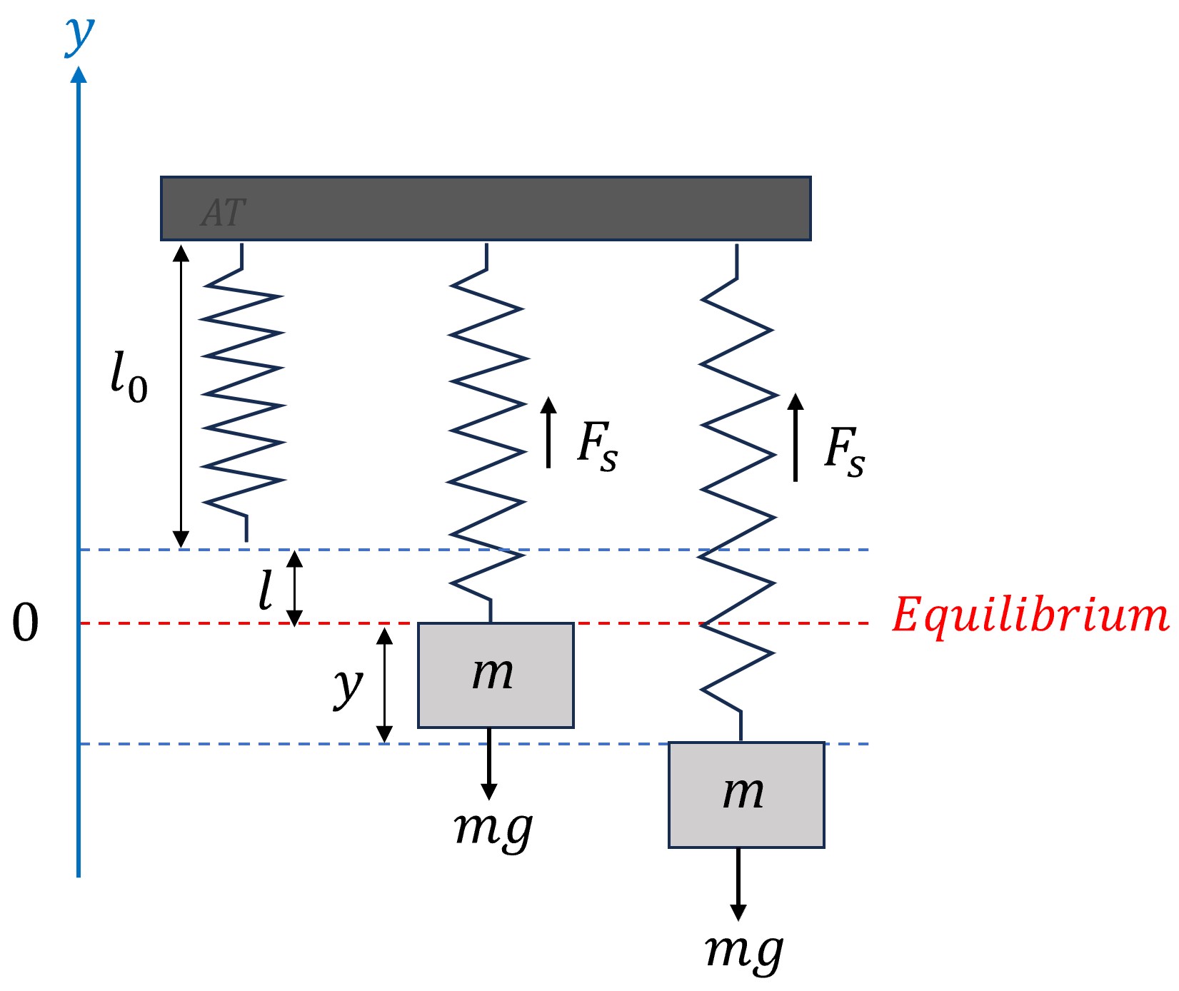
Consider the mass-spring system illustrated in Figure 3.8.1. The spring has a natural length of [asciimath]l_0[/asciimath] when unstretched. When we attach a mass [asciimath]m[/asciimath] to the spring, it stretches by a length [asciimath]l[/asciimath] . This point where the mass comes to rest and the spring ceases to stretch further is known as the equilibrium position. At this point, the system is stable, and the mass hangs motionless until disturbed. In this system, we define [asciimath]y[/asciimath] as the displacement of the mass from its equilibrium position, where positive values indicate upward movement.
To derive the equation governing the motion of a spring-mass-damper system, we apply Newton’s second law of motion, which relates the net force acting on the mass to its acceleration. The primary forces acting on the mass in a spring-mass system include:
According to Newton’s second law,
Substituting all the forces and writing acceleration as the second derivative of displacement yields
At equilibrium, the sum of all forces acting on the mass equals zero. Therefore,
Simplify the equation by incorporating [asciimath]mg=kl[/asciimath] to focus on deviations from equilibrium, leading to the standard form of the vibration equation.
[asciimath]my''+cy'+ky=F(t)[/asciimath] (3.8.1)
Here, [asciimath]y[/asciimath] is the displacement from the equilibrium position, [asciimath]y'[/asciimath] is the velocity, [asciimath]y''[/asciimath] is the acceleration, and [asciimath]F(t)[/asciimath] represents any external force applied to the system. We usually solve this equation along with the initial conditions for initial displacement from the equilibrium position: [asciimath]y(0)=y_0[/asciimath] and initial velocity: [asciimath]yprime (0)=y'_0[/asciimath] .
Depending on which forces act on the system, there are several special cases:
The simplest form of vibration occurs when there is no damping ( [asciimath]F_d=0[/asciimath] ) and no external force ( [asciimath]F(t)=0[/asciimath] ). In such cases, Equation 3.8.1 reduces to
[asciimath]my''+ky=0[/asciimath] (3.8.2)
This equation is a homogeneous second-order linear differential equation. By solving the characteristic equation [asciimath]mr^2+k=0[/asciimath] , we find that the roots are complex conjugates given by
The term [asciimath]sqrt(k/m)[/asciimath] is known as the natural frequency of the system, denoted by [asciimath]omega_0[/asciimath] . Therefore the solution to the equation is expressed as
[asciimath]y(t)=c_1cos(omega_0t)+c_2sin(omega_0t)[/asciimath] (3.8.3)
It is often convenient to represent the displacement in the amplitude-phase form with a single trigonometric function
[asciimath]y(t)=Rcos(omega_0t-phi)[/asciimath] (3.8.4)
Here [asciimath]R[/asciimath] is the amplitude of oscillation, given by [asciimath]R=sqrt(c_1^2+c_2^2)[/asciimath] and [asciimath]phi[/asciimath] is the phase angle, which can be determined from the initial conditions of the system. The phase angle [asciimath]phi[/asciimath] is typically chosen to satisfy [asciimath]-pilephiltpi[/asciimath] for uniqueness and is related to [asciimath]c_1[/asciimath] and [asciimath]c_2[/asciimath] .
[asciimath]cos(phi)=c_1/R=c_1/(sqrt(c_1^2+c_2^2))[/asciimath] and [asciimath]sin(phi)=c_2/R=c_2/(sqrt(c_1^2+c_2^2))[/asciimath]
The motion described by Equation 3.8.4 is known as simple harmonic motion, characterized by its sinusoidal nature and constant frequency. The period of the motion is [asciimath]T=(2pi)/(omega_0)[/asciimath] , representing the time it takes to complete one full cycle.
A 150 cm long vertical spring hangs from a fixed ceiling. A 2-kg object is attached to the lower end of the spring, and the length of the spring becomes 155 cm where the object is in equilibrium. The object is then pulled down an additional 3 cm and released with an initial upward velocity of 20 cm/s. Assuming no damping and no external forces other than gravity are acting on the system:
a) Find the displacement of the object as a function of time.
b) Determine the natural frequency, period, amplitude, and phase angle of the motion.
c) Rewrite the equation of motion in the amplitude-phase form [asciimath]y(t) = R cos(omega_0 t - phi)[/asciimath] .
Express your answers in the cgs unit where [asciimath]g=980\ "cm"//"s"^2[/asciimath] .
Show/Hide Solutiona)
Calculating the spring constant
At equilibrium, the forces acting on the object are balanced, meaning [asciimath]F_g=F_s[/asciimath] . This allows us to determine the spring constant [asciimath]k[/asciimath] .
Calculating the natural frequency:
The natural frequency is
It is important to note that to find [asciimath]omega_0[/asciimath] , we require the ratio of [asciimath]k[/asciimath] and [asciimath]m[/asciimath] rather than their individual values.
Finding the general solution:
Given there is no damping force and an external force, the initial value problem is
[asciimath]2y''+392y=0,[/asciimath] [asciimath]y_0(0)=-3,[/asciimath] [asciimath]y'_0(0)=20[/asciimath]
The general solution to this equation is given by Equation 3.8.3.
Applying the initial conditions:
The equation of the object displacement is then
b)
Natural frequency: [asciimath]omega_0=14 \ "rad"//"s"[/asciimath]
Period: [asciimath]T=(2pi)/(omega_0)=pi/7 \ "s"[/asciimath]
Amplitude [asciimath]R[/asciimath] is given by
Phase angle:
The reference phase angle is determined by
Since [asciimath]c_1lt0[/asciimath] ( [asciimath]cos(phi)lt0[/asciimath] ) and [asciimath]c_2gt0[/asciimath] ( [asciimath]sin(phi)gt0[/asciimath] ), [asciimath]phi[/asciimath] should be in the second quadrant. Therefore,
[asciimath]phi=pi-phi_R ~~ 2.697\ "rad"[/asciimath] .
c) The equation of motion can be written as
[asciimath]y(t) = R cos(omega_0 t - phi)[/asciimath]
[asciimath]y(t) = 1/7sqrt(541) cos(14 t - 2.697)[/asciimath]
The graph of the displacement is shown for the first 7 seconds.
Try an ExampleIn free, damped vibration, there is no external force ( [asciimath]F(t)=0[/asciimath] ). As such, Equation 3.8.1 simplifies to a homogeneous second-order linear differential equation.
[asciimath]my''+cy'+ky=0[/asciimath] (3.8.5)
This equation is a homogeneous second-order linear differential equation. By solving the characteristic equation [asciimath]mr^2+cr+k=0[/asciimath] using the quadratic formula, we find the roots
Depending on the discriminant [asciimath]c^2-4mk[/asciimath] , we encounter three types of motion:
1. Critically damped ( [asciimath]c^2-4mk=0[/asciimath] )
In this case, there is a repeated root [asciimath]r=-c/(2m)[/asciimath] , and thus the general solution to Equation 3.8.5 becomes
[asciimath]y(t)=c_1e^(-c/(2m)t)+c_2te^(-c/(2m)t)[/asciimath] (3.8.6)
The motion in this case is said to be critically damped as the damping is just enough to prevent oscillation. This level of damping is achieved when the damping coefficient [asciimath]c[/asciimath].
[asciimath]2sqrt(mk)[/asciimath] is called the critical damping coefficient and is denoted by [asciimath]C_(cr)[/asciimath] .
It is important to note that as time progresses ( [asciimath]trarroo[/asciimath] ), the displacement [asciimath]y(t)[/asciimath] approaches zero, indicating that the system smoothly and quickly settles to its equilibrium position without oscillation and overshooting the equilibrium position similar to how shock absorbers work in automotive suspension systems.
2. Overdamped ( [asciimath]c^2-4mkgt0[/asciimath] )
In this case, there are two real distinct roots [asciimath]r_(1,2)=(-c+-sqrt(c^2-4mk))/(2m)[/asciimath] , where both roots are negative. The general solution to Equation 3.8.5 becomes
[asciimath]y(t)=c_1e^(r_1t)+c_2e^(r_2t)[/asciimath] (3.8.7)
Given both [asciimath]r_1[/asciimath] and [asciimath]r_2[/asciimath] are negative, as time progresses ( [asciimath]trarroo[/asciimath] ), the displacement [asciimath]y(t)[/asciimath] approaches zero and the system gradually returns to equilibrium without oscillating. Overdamped conditions arise when [asciimath]cgtc_(cr)[/asciimath] , typically desired in systems where overshooting the equilibrium position could be harmful or undesirable, like in heavy machinery. Overdamped systems return to equilibrium slower than critically damped systems. This slower response is due to the higher damping force applied, which prevents oscillation but also resists motion, causing a sluggish return.
3. Underdamped ( [asciimath]c^2-4mklt0[/asciimath] )
In this case, the roots of the characteristic equation are complex conjugates given by
Thus the solution to the differential Equation 3.8.5 is
[asciimath]y(t)=e^(-c/(2m)t)(c_1cos(omega_1t)+c_2sin(omega_1t))[/asciimath] (3.8.8)
The term [asciimath]omega_1=(sqrt(4mk-c^2))/(2m)[/asciimath] is related to the frequency of oscillation. Similar to the harmonic motion, we can derive the amplitude-phase form of the equation of motion.
[asciimath]y(t)=Re^(-c/(2m)t)cos(omega_1t-phi)[/asciimath] (3.8.9)
[asciimath]R=sqrt(c_1^2+c_2^2)[/asciimath] , [asciimath]cos(phi)=(c_1)/R[/asciimath] , and [asciimath]sin(phi)=(c_2)/R[/asciimath]
An underdamped system is characterized by a damping coefficient [asciimath]cltc_(cr)[/asciimath] . In this scenario, the damping is insufficient to halt oscillations, causing the system to exhibit oscillatory behavior around the equilibrium position. The amplitude of these oscillations diminishes over time, represented by the time-varying term [asciimath]Re^(-c/(2m)t)[/asciimath] . As the exponent [asciimath]-c/(2m)[/asciimath] is always negative, the displacement [asciimath]y(t)[/asciimath] gradually approaches zero as time progresses ( [asciimath]trarroo[/asciimath] ). This results in a bouncy system response to any disturbances.
Such behavior is often preferred in various applications. In musical instruments, for example, the underdamped vibrations of strings or membranes contribute to a sustained, resonant sound. Similarly, seismic dampers in buildings employ a controlled underdamped response to safely dissipate energy from earthquakes, allowing structures to sway and reduce stress without collapsing.
Example 3.8.2: Critically Damped MotionA 1-kg mass is attached to a string with a stiffness of 64 N/m and a dashpot with a damping constant 16 N.s/m. The object is compressed 20 cm above its equilibrium and released with an initial upward velocity of 2 m/s. Find the displacement of the object as a function of time.
Show/Hide SolutionThe initial value problem for this system is
[asciimath]y''+16y'+64y=0,[/asciimath] [asciimath]y_0(0)=0.2,[/asciimath] [asciimath]y'_0(0)=2[/asciimath]
Before solving the IVP, we can calculate the critical damping coefficient to determine the type of damping.
The damping coefficient equals the critical damping coefficient ( [asciimath]c=c_(cr)=16[/asciimath] ), and therefore, the system is critically damped.
Finding the general solution:
The general solution for a critically damped system is given by Equation 3.8.6.
Applying the initial conditions:
The equation of the object’s displacement is then
The graph of the displacement is shown for the first 3 seconds. As expected, the system smoothly and quickly returns to its equilibrium position without oscillation.

Find the displacement of the object in Example 3.8.2, if the spring is now attached to a dashpot with a damping constant 34 N.s/m.
Show/Hide SolutionThe initial value problem for this system is
[asciimath]y''+34y'+64y=0,[/asciimath] [asciimath]y_0(0)=0.2,[/asciimath] [asciimath]y'_0(0)=2[/asciimath]
In the previous example, we determined the critical damping coefficient to be [asciimath]c_(cr)=16[/asciimath] . In the current system, the damping coefficient is greater than this critical value ( [asciimath]c>c_(cr)=16[/asciimath] ), and therefore, the system is overdamped.
Finding the general solution:
The characteristic equation for the differential equation has two distinct real roots.
The general solution to an overdamped system is given by Equation 3.8.7.
Applying the initial conditions:
Solving the system for constants [asciimath]c_1[/asciimath] and [asciimath]c_2[/asciimath] yields
The equation of the object’s displacement is then
The below graph displays the displacement for the first 3 seconds. It confirms that the system gradually returns to its equilibrium position smoothly and without any oscillation. When compared to the critically damped system in Example 3.8.2, this overdamped system takes a longer time to settle down. This slower behavior underscores that the increased damping force in the overdamped system delays the return to equilibrium.

Find the displacement of the object in Example 3.8.2, if the spring is now attached to a dashpot with a damping constant 4 N.s/m.
Show/Hide SolutionThe initial value problem for this system is
[asciimath]y''+4y'+64y=0,[/asciimath] [asciimath]y_0(0)=0.2,[/asciimath] [asciimath]y'_0(0)=2[/asciimath]
In Example 3.8.2, we determined the critical damping coefficient to be [asciimath]c_(cr)=16[/asciimath] . In the current system, the damping coefficient is less than this critical value ( [asciimath]cltc_(cr)=16[/asciimath] ), and therefore, the system is underdamped.
Finding the general solution:
The characteristic equation for the differential equation has complex conjugates.
The general solution to an underdamped system is given by Equation 3.8.8.
Applying the initial conditions:
[asciimath]y'(t)=e^(-2t)(-2c_1cos(2sqrt(15)t)-2c_2sin(2sqrt(15)t)-[/asciimath] [asciimath]2sqrt(15) c_1sin(2sqrt(15)t)+2sqrt(15) c_2cos(2sqrt(15)t))[/asciimath]
The equation of the object’s displacement is then
The amplitude-phase form of the equation is
The graph illustrates the displacement of the system over the initial 3 seconds. This underdamped system lacks enough damping to stop oscillations, leading to a pattern of diminishing swings around the equilibrium position. These oscillations decrease in amplitude for approximately 2 seconds before the system finally settles at the equilibrium position.

Forced undamped vibration occurs in systems subject to a continuous external force, typically modeled as a periodic function like [asciimath]F(t)=F_0 cos(omega t)[/asciimath] or [asciimath]F(t)=F_0 sin(omega t)[/asciimath] . These sinusoidal forces commonly arise from rotational mechanisms, alternating currents, or other cyclic phenomena. The equation of motion for such a system is expressed as
The solution to the differential equation is
[asciimath]y(t)=y_p (t)+y_c (t)[/asciimath]
Here, the solution comprises a complementary part [asciimath]y_c(t)[/asciimath] , representing the free, undamped vibration response, and a particular part [asciimath]y_p(t)[/asciimath] , the steady-state response to the forcing function. The complementary solution, dictated by the system’s natural frequency [asciimath]omega_0=k/m[/asciimath] , is given by Equation 3.8.3:
To determine the particular solution, we typically use methods like undetermined coefficients or variation of parameters. As we seek the particular solution, depending on the driving frequency omega, we consider two cases:
1. Non-Resonant ( [asciimath]omega!=omega_0[/asciimath] ): When the driving frequency is different from the natural frequency, the particular solution is in the form
To find the specific values of the coefficients A and B, we use the method of undetermined coefficients. After determining these coefficients, the particular solution can be expressed as
and the general solution is
[asciimath]y(t)=F_0/(m(omega_0^2-omega^2))cos(omega t)+[/asciimath] [asciimath]c_1cos(omega_0t)+c_2sin(omega_0t)[/asciimath] (3.8.10)
The displacement function consists of sine and cosine components with bounded amplitude.
2. Resonant ( [asciimath]omega=omega_0[/asciimath] ): When the driving frequency is equal to the natural frequency, the particular solution is in the form
using the method of undetermined coefficients and after determining the coefficients, the particular solution can be expressed as
[asciimath]y_p=F_0/(2m omega_0)t sin(omega_0 t)[/asciimath]
The general solution is then
[asciimath]y(t)=F_0/(2m omega_0)t sin(omega_0 t)+[/asciimath] [asciimath]c_1cos(omega_0t)+c_2sin(omega_0t)[/asciimath] (3.8.11)
In this case, the particular solution includes a time factor [asciimath]t[/asciimath] , indicating the unbounded increase in amplitude. This phenomenon, known as resonance, significantly increases oscillation amplitude and poses potential risks, including mechanical failure from excessive oscillations.
The amplitude of oscillation in forced vibration is sensitive to the relationship between the driving frequency and the natural frequency of the system. As the driving frequency approaches the natural frequency, the amplitude increases, peaking at resonance. This sensitivity is a key factor in designing structures and systems to ensure their natural frequencies are not aligned with frequencies of common environmental forces, like wind or traffic. Such alignment could trigger resonance, risking structural integrity.
On the other hand, there are specific applications where inducing resonance is advantageous, for instance, in mechanical filters and sensors, where resonance can enhance sensitivity or signal strength.
Example 3.8.5: Forced Undamped VibrationA 32 lb object is suspended from a spring, stretching it by 6 inches to reach equilibrium. This undamped system is subjected to an external force [asciimath]F(t) = 2cos(8t)[/asciimath], and it experiences resonance. Initially, the object is displaced 3 inches below the equilibrium position and is given an upward velocity of 1 ft/s. Determine the object’s displacement under these conditions.
Show/Hide SolutionCalculating the spring constant
In the British system, weight is typically measured in pounds. To find the spring constant, we first convert weight to mass using the formula
At equilibrium [asciimath]F_g=F_s[/asciimath] . This relationship allows us to calculate the spring constant [asciimath]k[/asciimath] .
[asciimath]mg=k( l) ->\ k=(mg)/( l)[/asciimath]
Calculating the natural frequency:
The natural frequency is
Alternatively, if the system resonates at a driving frequency of [asciimath]omega=8[/asciimath] (from [asciimath]F(t) = 2 cos(8t)[/asciimath] ), this resonance frequency should match the natural frequency of the system, reaffirming that [asciimath]omega_0=8[/asciimath] .
Finding the general solution:
The initial value problem for this system is
[asciimath]y''+64y=2cos(8t),[/asciimath] [asciimath]y_0(0)=-0.25,[/asciimath] [asciimath]y'_0(0)=1[/asciimath]
The general solution for a system undergoing resonance is given by Equation 3.8.11.
[asciimath]y(t)=2/(2(1)(8))t sin(8 t)+c_1cos(8t)+c_2sin(8t)[/asciimath]
[asciimath]y(t)=1/8t sin(8 t)+c_1cos(8t)+c_2sin(8t)[/asciimath]
Applying the initial conditions:
[asciimath]y_0(0)=-0.25 \ ->[/asciimath] [asciimath]c_1=-0.25=-1/4[/asciimath]
[asciimath]y'_0(0)=1\ ->[/asciimath] [asciimath]c_2=0.125=1/8[/asciimath]
The equation of the object’s displacement is then
[asciimath]y(t)=1/8t sin(8 t)-1/4cos(8t)+1/8sin(8t)[/asciimath]
We can write the complementary solution in the amplitude-phase form, combining the last two terms.
The graph shows how the system’s displacement changes during the first 10 seconds. Since the particular solution includes a time factor (t), the displacement’s amplitude tends to become infinitely large as time progresses towards infinity. However, in reality, most systems experience some damping. Even a small amount of damping can significantly affect the system’s amplitude and behavior, especially around resonance frequencies, preventing the unlimited growth in amplitude predicted by ideal models.

This is the most general case, combining the effects of damping and external forcing. The motion of such a system is governed by
The solution to the differential equation is the sum of complementary and particular solutions.
[asciimath]y(t)=y_p (t)+y_c (t)[/asciimath]
The complementary solution is the solution to the free, damped behavior, while the particular solution is found using the method of undetermined coefficients or variation of parameters.
Based on our understanding of free-damped vibrations, we know that as time progresses toward infinity, the complementary solution approaches zero. Consequently, the system’s displacement increasingly reflects the behavior of the particular solution. Therefore, in vibrational analysis, the complementary solution is commonly referred to as the transient solution, reflecting the initial response, while the particular solution is known as the steady-state solution, indicating the ongoing response to the external force.
Example 3.8.6: Forced Damped VibrationFind the displacement of the object in Example 3.8.5, if the system is now attached to a dashpot with a damping constant 34 lb.s/ft.
Show/Hide SolutionIn the previous example, we determined the spring constant: [asciimath]k=64\ "lbf/ft"[/asciimath] . The initial value problem for this system is
[asciimath]y''+20y'+64y=2cos(8t),[/asciimath] [asciimath]y_0(0)=-0.25,[/asciimath] [asciimath]y'_0(0)=1[/asciimath]
Given the characteristic equation has distinct real roots [asciimath]r_1=-4[/asciimath] and [asciimath]r_2=-16[/asciimath] , the complementary solution, according to Equation 3.8.7, is
Finding the particular solution:
To find the particular solution, we use undetermined coefficients. Given the forcing cosine function, we guess the form of the particular solution to be
The derivatives are
Substituting [asciimath]Y_p[/asciimath] and its derivatives into the differential equation yields
Simplifying it gives
By matching coefficients of sine and cosine terms, we get
Therefore, the particular solution is
Combining the particular and complementary solutions gives the general solution
Applying the initial conditions:
[asciimath]y_0(0)=-0.25 \ ->[/asciimath] [asciimath]c_1+c_2=-1/4[/asciimath]
[asciimath]y'_0(0)=1\ ->[/asciimath] [asciimath]-4c_1-16c_2=9/10[/asciimath]
Solving the system, we find the constants to be
The equation of the object’s displacement is then
The graph depicts the change in the system’s displacement over the first 6 seconds. Initially, for about the first second, the displacement is primarily influenced by the complementary solution, reflecting the transient phase. After this initial period, the displacement increasingly aligns with the periodic particular solution, representing the steady-state behavior of the system.

a) [asciimath]k=588[/asciimath] N/m b) [asciimath]y(t)=1/10cos(7sqrt(6)t)+2/(7sqrt(6))sin(7sqrt(6)t)[/asciimath]
Show/Hide Answera) [asciimath]y(t)=e^(-9/26t)(5cos(sqrt(387)/(26)t)+45/sqrt(387)sin(sqrt(387)/(26)t))[/asciimath] b) Free underdamped vibration